





Editorial Integrity
Making informed real estate decisions starts with having the right knowledge. At HomeAbroad, we offer US mortgage products for foreign nationals & investors and have a network of 500+ expert HomeAbroad real estate agents to provide the expertise you need. Our content is written by licensed mortgage experts and seasoned real estate agents who share insights from their experience, helping thousands like you. Our strict editorial process ensures you receive reliable and accurate information.
Typical single-family rent and median household income often support different mortgage rates.
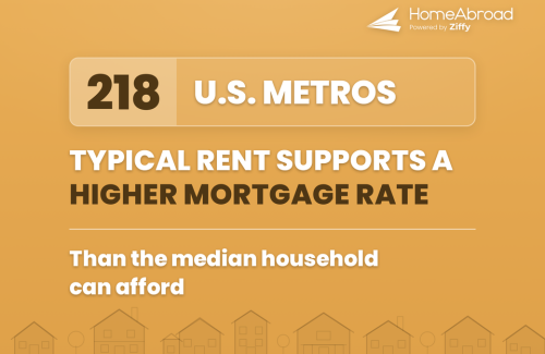
In 218 of 375 U.S. metros analyzed, typical single-family rent supports a higher 30-year mortgage rate than median household income does. At the study’s 6.58% benchmark, 209 metros clear neither the rent-coverage nor household-income test, while 30 clear only the rent test.
Because that income is measured in 2024 while home values and rents are from June 2026, the count is sensitive to the income vintage: raising income 3% lowers it to 185 metros, and a CPI translation to June 2026 dollars lowers it to 153. The 218 figure is therefore tied to the published 2024 estimate, and the more durable finding is the directional divergence between rents and local incomes rather than the size of the national majority.
The analysis solves for the highest mortgage rate at which a typical single-family home passes each test, assuming a 20% down payment, a 30-year mortgage, and standardized property tax and insurance costs. It uses June 2026 Zillow home values and rents and the latest available 2024 Census ACS median household income.
Table of Contents
In 22 of 26 metros where household income fails even at 0%, rent still supports a positive mortgage rate
In these markets, lowering rates cannot make the typical home affordable to the median-income household under the model, but the typical single-family rent can still support financing. Only four metros fail both tests at every nonnegative rate.
Buyers and rents point in opposite directions in 69 metros at the 6.58% benchmark
Thirty metros pass only the rent-coverage test, while 39 pass only the household-income test. The similar national totals -127 rent-supported and 136 income-supported hide substantial local differences in which side can carry the modeled payment.
Miami’s typical rent supports 5.89%, even though median household income supports no nonnegative rate
Miami is one of the clearest local examples of the divide. The median-income household cannot meet the modeled affordability threshold even at 0% interest, while typical single-family rent supports a rate only 0.69 percentage points below the study benchmark.
In 69 U.S. Metros, Rent and Local Incomes Point to Opposite Housing Markets
At the same mortgage rate, a home can produce very different affordability results depending on who is carrying the payment.
A median-income household must keep modeled principal, interest, taxes and insurance within 30% of income. A rental property passes a different test: whether typical single-family rent covers the same modeled monthly payment.
At the study’s 6.58% benchmark, those tests agree in most metros but not always. In 97 metros, both rent and household income support the payment. In 209, neither does. The more revealing group is the 69 metros where the two tests point in opposite directions:
-
 In 30 metros, typical rent covers the payment even though the median household cannot.
 - In 39 metros, the median household can afford the payment even though typical rent does not fully cover it.
That split shows why national affordability counts can hide very different local market conditions. Two metros may have similar home values and mortgage costs but produce opposite outcomes depending on local wages and rents.

Amresh Singh
Founder and CEO | Ziffy & HomeAbroad
For years, affordability has been framed around what the local buyer can pay. This analysis shows that in most metros the typical rent and the median paycheck are answering two different questions about the same home and in 69 of them they point in opposite directions. That divergence, not the national average, is where the real story is.
The Four Positions at the 6.58% Benchmark
Position | What it means | Metros | Share |
|---|---|---|---|
Both tests clear | Rent covers the payment and modeled PITI remains within the household-income ceiling | 97 | 25.9% |
Rent clears first | Rent covers the payment, but the household-income test does not | 30 | 8.0% |
Income clears first | The household-income test clears, but rent does not cover the payment | 39 | 10.4% |
Neither test clears | Both require a mortgage rate below 6.58% | 209 | 55.7% |
Total | 375 | 100% |
Note: These are positions at one common benchmark, not permanent market labels. Metros close to 6.58% can move between groups with small changes in rates, taxes, insurance, rents or income. The report therefore publishes each metro’s exact solved rate and uses 6.58% only as a consistent national comparison point.
Rent vs. Household-Income Mortgage Rate Statistics [375 Metros Analyzed]
-
 A lender-style rent test cuts the number of viable metros from 127 to just 28
At the 6.58% benchmark, typical rent covers the modeled payment in 127 metros. Requiring rent to equal 120% of that payment reduces the count to only 28 metros, or 7.5%, while 20 metros fail the 1.20x test even at 0% interest. - The typical metro has a 1.37-percentage-point gap between its rent- and income-supported rates
The national average gap appears close to zero only because positive and negative metro gaps offset. In the typical metro, the absolute difference is 1.37 percentage points, and only 22.1% of metros have the two solved rates within half a point of each other. - Pittsfield and Ithaca have rent-supported rates more than five points above their income-supported rates
Among metros stable across the published sensitivity tests, Pittsfield’s rent-supported rate is 8.51%, compared with 3.41% from household income. Ithaca shows a similar divide: 8.73% versus 3.72%. - In the West, rent is usually the stronger anchor- even though almost no metro clears the benchmark
The rent-supported rate exceeds the income-supported rate in 70 of 85 Western metros, yet 84 of the 85 clear neither test at 6.58%. Rent is stronger relative to income, but generally not strong enough to make current pricing work at the benchmark. - The Midwest shows the opposite pattern: local incomes outperform rents
In the Midwest, 26 metros clear only the household-income test, compared with just four that clear only the rent test. Detroit and St. Louis are major examples where local-buyer affordability works at the benchmark but typical rent does not cover the modeled payment. - Detroit and St. Louis support high buyer-affordability rates but weaker rental coverage
Detroit’s household-supported rate is 7.70%, while its rent-supported rate is 5.97%. In St. Louis, the divide is wider: 7.88% from household income versus 5.59% from rent. - Chicago and Dallas sit just across the rent-first line
In Chicago, typical rent supports 7.21%, while household income supports 5.67%. Dallas is much closer to the benchmark, with rent supporting 6.64% and income supporting 6.28%, showing how small local differences can place buyers and rental math on opposite sides of the same rate. - New Orleans and Lakeland remain clear rent-first markets even under the stability tests
New Orleans supports an 8.05% rent-based rate versus 5.41% from household income. Lakeland supports 7.64% from rent and 4.79% from income. Both remain in the rent-first category across the published benchmark sensitivities. - At rates below 5%, rent clears more metros than household income does
At a 3% mortgage rate, typical rent covers the modeled payment in 333 metros, compared with 298 that pass the household-income test. At 5%, the counts are 236 versus 214. The advantage disappears only as rates approach the 6.58% benchmark. - Five metros cannot support the modeled payment from rent even at 0%
San Francisco, San Jose, Urban Honolulu, Barnstable Town and Sheboygan have no nonnegative rent-side solution. In the first four, neither typical rent nor median household income supports the modeled payment at any nonnegative mortgage rate; Sheboygan is the exception, where household income clears but rent does not.
Note: For the direction of the gap alone, the test is simple: rent supports the higher rate whenever typical monthly rent exceeds 2.5% of annual median household income (30% over 12 months). The mortgage-rate framing adds what that ratio can’t – the level of each rate, the gap size, no-solution markets, and each metro’s position at 6.58%.
How the Largest U.S. Metros Compare on Rent and Buyer Affordability
The national pattern becomes more tangible in the country’s largest housing markets. Among the 25 largest metros, only Houston and San Antonio clear both the rent and household-income tests at the study’s 6.58% benchmark.
Chicago and Dallas-Fort Worth fall on the rental-first side: typical rent covers the modeled payment, but the median household-income test does not. Detroit and St. Louis show the opposite pattern, with household income supporting the benchmark while typical rent falls short.
Most large coastal and high-cost metros clear neither test. New York, Los Angeles and Miami have no household-income solution at any nonnegative rate, although their typical rents still support positive mortgage rates. In San Francisco, neither household income nor typical rent covers the modeled payment even at 0% interest.
These positions show that high home values do not produce one uniform result. Some metros are constrained primarily by local incomes, some by rent coverage, and many by both.
Metro | Household-supported rate | Rent-supported rate | Position at 6.58% | Stability |
|---|---|---|---|---|
New York | No solution ≥0% | 3.15% | Neither | Stable |
Los Angeles | No solution ≥0% | 2.20% | Neither | Stable |
Chicago | 5.67% | 7.21% | Rent clears first | Can change |
Dallas–Fort Worth | 6.28% | 6.64% | Rent clears first | Can change |
Houston | 6.73% | 7.95% | Both clear | Can change |
Miami | No solution ≥0% | 5.89% | Neither | Stable |
Washington, D.C. | 3.66% | 4.34% | Neither | Stable |
Atlanta | 5.58% | 5.53% | Neither | Stable |
Philadelphia | 4.96% | 5.40% | Neither | Stable |
Phoenix | 3.51% | 3.83% | Neither | Stable |
Boston | 0.53% | 3.73% | Neither | Stable |
Riverside | 0.74% | 4.38% | Neither | Stable |
San Francisco | No solution ≥0% | No solution ≥0% | Neither | Stable |
Detroit | 7.70% | 5.97% | Income clears first | Can change |
Seattle | 0.07% | 2.44% | Neither | Stable |
Minneapolis | 5.73% | 5.82% | Neither | Stable |
Tampa | 4.07% | 6.577% | Neither | Can change |
San Diego | No solution ≥0% | 1.72% | Neither | Stable |
Denver | 2.54% | 3.75% | Neither | Stable |
Orlando | 3.70% | 6.07% | Neither | Can change |
Charlotte | 4.61% | 4.93% | Neither | Stable |
Baltimore | 5.50% | 5.59% | Neither | Stable |
St. Louis | 7.88% | 5.59% | Income clears first | Stable |
San Antonio | 7.50% | 6.93% | Both clear | Can change |
Austin | 5.26% | 4.41% | Neither | Stable |
Note: “Stable” means the benchmark position remains unchanged across the report’s income, rent and standardized-cost sensitivity tests. “Can change” means at least one tested scenario moves the metro into another benchmark position.
The Largest Metros Where Rent Clears but Household Income Does Not
The rental-first group includes two of the five largest U.S. metros: Chicago and Dallas-Fort Worth. The divide is wider in several smaller markets, including New Orleans, Lakeland and Springfield, Massachusetts.
Metro | Household-supported rate | Rent-supported rate | Difference |
|---|---|---|---|
Chicago | 5.67% | 7.21% | 1.54 pp |
Dallas-Fort Worth | 6.28% | 6.64% | 0.35 pp |
Buffalo | 5.96% | 7.12% | 1.16 pp |
New Orleans | 5.41% | 8.05% | 2.63 pp |
El Paso | 6.50% | 8.65% | 2.15 pp |
Lakeland | 4.79% | 7.64% | 2.85 pp |
Greensboro | 5.86% | 7.30% | 1.44 pp |
Port St. Lucie | 3.76% | 7.10% | 3.34 pp |
Springfield, Massachusetts | 2.74% | 6.75% | 4.01 pp |
A metro appearing in this group does not necessarily offer positive investment cash flow. The rent test measures whether typical rent covers the standardized PITI payment before vacancy, maintenance, capital expenditures, management and other operating costs.
Only 28 Metros Clear a Stricter 1.20x Rent-Coverage Test
The analysis primary rent-supported rate uses a 1.00x threshold: typical rent must equal the modeled principal, interest, property tax and insurance payment.
That is useful for comparing rent with household income on the same payment basis, but it leaves no allowance for operating expenses. To test how quickly the results narrow when more headroom is required, the analysis also applies a 1.20x gross-rent coverage standard, meaning rent must equal 120% of modeled PITI.
At the 6.58% benchmark:
| Rent-coverage standard | Metros clearing | Share |
| Rent equals modeled PITI, 1.00x | 127 | 33.9% |
| Rent equals 120% of modeled PITI, 1.20x | 28 | 7.5% |
The stricter requirement removes 99 of the 127 metros that clear the basic rent test. Put differently, nearly four in five metros that cover standardized PITI do not generate an additional 20% of gross-rent headroom at the same rate.
The effect is visible even in major rental-first markets. Chicago’s rent-supported rate falls from 7.21% under the primary test to 5.03% at 1.20x. Dallas-Fort Worth falls from 6.64% to 4.49%, while New Orleans falls from 8.05% to 5.79%.
Twenty metros have no 1.20x solution even at 0% interest. In those markets, typical rent does not reach 120% of the modeled payment even after financing costs are removed.
The 1.20x test remains a standardized market-comparison measure, not a lender underwriting result. It does not incorporate property-specific rent, taxes, insurance, vacancy, maintenance or loan terms, and it should not be interpreted as a DSCR qualification determination.
Lower Rates Help Both Sides, but Rent Leads Until About 5%
The 6.58% benchmark provides one common snapshot, but the relationship changes as mortgage rates fall. At every modeled rate below 5%, typical rent covers the payment in more metros than the household-income test clears. At 3%, rent covers modeled PITI in 333 metros, while the income test clears in 298. At 5%, the difference narrows to 236 versus 214.
Near the study benchmark, however, the two national totals converge and eventually reverse slightly. At 6.58%, rent covers the modeled payment in 127 metros, compared with 136 where PITI remains within 30% of median household income.
Modeled mortgage rate | Rent covers modeled PITI | PITI stays within income ceiling | Rent covers PITI at 1.20x |
|---|---|---|---|
0% interest | 370 | 349 | 355 |
2.00% | 354 | 320 | 293 |
3.00% | 333 | 298 | 233 |
4.00% | 291 | 258 | 159 |
5.00% | 236 | 214 | 94 |
6.58% | 127 | 136 | 28 |
The pattern does not mean rent is universally stronger. It means that, across the analyzed metros, the rent side reaches a workable payment in more markets when financing costs are lower. As rates approach the benchmark, the number of metros clearing either test falls sharply and the two national totals become similar.
The stricter 1.20x standard declines much faster. Although 355 metros meet it at 0% interest, only 94 do at 5%, and just 28 at 6.58%.
The Headline Result Is Sensitive to Income Timing, but the Broader Divide Remains
The headline comparison combines June 2026 home values and rents with the latest available metro-level household-income data from the 2024 ACS. Because those inputs come from different periods, the report tests how the result changes when income, rent and standardized housing costs are varied.
The central finding – rent supporting the higher rate in 218 metros is not equally strong under every scenario. The precise count changes materially, and the report should state that prominently rather than treating sensitivity as a technical appendix.

Debjit Saha
Co-Founder and CTO | Ziffy & HomeAbroad
We built this to be checkable – one standardized model, every rate solved numerically and independently rebuilt row by row. The direction of the divide is what holds: the 218-metro majority moves with the income vintage, but rents and local incomes diverge across every scenario we tested. That’s the finding we’d stand behind.
Updating income toward 2026 removes the national majority
Using published 2024 ACS income, rent supports the higher rate in 218 metros, or 58.1%.
When income is raised to approximate a later period, the count falls:
| Income assumption | Metros where rent supports the higher rate | Share |
| Published 2024 ACS income | 218 | 58.1% |
| Income increased by 3% | 185 | 49.3% |
| Income increased by 5% | 164 | 43.7% |
| CPI-translated to June 2026 dollars | 153 | 40.8% |
The headline majority therefore applies specifically to the published 2024 income estimate. It does not survive the illustrative higher-income scenarios.
These scenarios are not estimates of actual 2026 metro income. They show how strongly the comparison depends on the income vintage until newer ACS metro data become available
Census sampling uncertainty also moves the count
Median household income is an ACS estimate with a published margin of error. Recalculating the model at each metro’s lower and upper income bounds produces a wide national range.
| ACS income assumption | Rent rate exceeds income rate | Income test clears at 6.58% | No income solution at 0% |
|---|---|---|---|
| Lower income bound | 261 | 109 | 32 |
| Published estimate | 218 | 136 | 26 |
| Upper income bound | 168 | 163 | 17 |
Rent supports the higher rate in more metros when household income is placed at the lower end of its ACS range and in fewer metros when income is placed at the upper end.
These are scenario bounds, not statistical confidence intervals for the national count.
A 5% change in rent can erase or expand the majority
Because Zillow’s rent measure is a smoothed index of typical asking rents, the report also tests rents 5% above and below the central value.
| Rent assumption | Rent rate exceeds income rate | Rent clears at 6.58% | No rent solution at 0% |
|---|---|---|---|
| Rent −5% | 162 | 92 | 6 |
| Published rent | 218 | 127 | 5 |
| Rent +5% | 256 | 166 | 2 |
A 5% rent reduction lowers the headline count from 218 to 162, so the majority does not survive the lower-rent scenario. A 5% increase raises it to 256.
Tax and insurance affect benchmark classifications more than the gap direction
The primary model uses standardized annual property tax of 1.1% of home value and homeowners insurance of 0.5%. Varying the combined cost from 1.2% to 2.2% changes the number of metros clearing the 6.58% benchmark substantially.
| Combined annual tax and insurance | Rent rate exceeds income rate | Rent clears at 6.58% | Income clears at 6.58% | Rent clears first |
|---|---|---|---|---|
| 1.2% of value | 221 | 167 | 161 | 43 |
| 1.6% base assumption | 218 | 127 | 136 | 30 |
| 2.2% of value | 212 | 82 | 104 | 20 |
The broader question of which side supports the higher rate changes relatively little, from 212 to 221 metros. The four-way benchmark classifications change much more because many metros sit close to 6.58%.
This distinction matters: the direction of the rent-versus-income gap is more stable than the exact position of many metros at one benchmark rate.
Most Metros Keep Their Broad Direction, but Many Move Across the Benchmark
To prevent close calls from being presented as firm rankings, the analysis assigns two stability measures to every metro.
Gap-direction stability asks whether rent continues to support a higher rate—or income continues to support a higher rate – across all published one-factor scenarios.
Benchmark-position stability asks whether the metro remains in the same four-way group at 6.58%: both clear, rent only, income only or neither.
Across the 375 metros:
| Stability measure | Stable metros | Share |
|---|---|---|
| Gap direction remains unchanged | 248 | 66.1% |
| Four-way benchmark position remains unchanged | 240 | 64.0% |
Of the 218 metros where rent supports the higher rate in the central model, 141 remain rent-led across every tested scenario, while 77 can reverse under at least one assumption.
The report should use only metros stable on both measures for claims such as “largest gap” or “strongest divide.” Metros close to the benchmark may still be useful examples, but their sensitivity should be shown directly.
The national result is also largely unchanged when the four Connecticut metros with unresolved geographic-footprint compatibility are removed: rent supports the higher rate in 214 of 371 metros, or 57.7%.
In 97 Metros, Both Rent and Household Income Support the Benchmark
The report’s central story is the divergence between rents and local incomes, but nearly one-quarter of the analyzed metros produce a more favorable result.
In 97 metros, or 25.9%, typical single-family rent covers modeled PITI at 6.58% and the same payment remains within 30% of median household income.
These markets are concentrated in lower-value areas where the standardized model leaves enough payment room on both sides. Among larger metros, Houston and San Antonio fall into this group. Pittsburgh, Indianapolis, Cleveland, Memphis and Rochester, New York, also clear both tests.
| Selected metro | Household-supported rate | Rent-supported rate |
|---|---|---|
| Pittsburgh | 9.83% | 8.27% |
| Indianapolis | 6.95% | 6.70% |
| Cleveland | 7.42% | 6.96% |
| Memphis | 7.42% | 7.06% |
| Rochester, NY | 6.82% | 8.76% |
| San Antonio | 7.50% | 6.93% |
| Houston | 6.73% | 7.95% |
Passing both tests does not mean every home in the metro is affordable or produces positive investment cash flow. It means the typical metro-level value passes both standardized payment tests under the study’s assumptions
Methodology
Data Sources
This analysis uses four primary data inputs.
1. Typical single-family home values
Zillow’s Home Value Index for single-family homes supplied the June 2026 metro-level home values used in the model.
ZHVI measures the typical value of homes within the selected housing category. It is not a median sale price, an asking price or the value of a particular property. Changes in the index should not be interpreted as changes in the price of every home within a metro.
2. Typical single-family rents
Zillow’s Observed Rent Index for single-family residences supplied the June 2026 metro-level rents.
ZORI is a smoothed measure of typical asking rent weighted to the rental housing stock. It does not represent the rent paid under an existing lease, the rent achieved by every property or the rent of the same physical home represented by the ZHVI value.
The value and rent inputs are matched by Zillow metro identifier, property category and observation month.
3. Median household income
Median household income came from the U.S. Census Bureau’s 2024 American Community Survey one-year estimates, table B19013.
The analysis uses the central estimate and its published 90% margin of error. Income is reported in 2024 inflation-adjusted dollars and is the latest available ACS metro-level income release covering the study universe.
4. Mortgage-rate benchmark
The study benchmark is Freddie Mac’s 6.58% average 30-year fixed mortgage rate for the week ending July 23, 2026.
The benchmark describes a national owner-occupied mortgage market and is used only as a common comparison rate. It is not an investor mortgage quote, a DSCR rate or a forecast of future borrowing costs.
Metro Universe and Coverage
The starting universe contains 387 U.S. metropolitan statistical areas under the July 2023 Office of Management and Budget delineations, excluding Puerto Rico.
A metro is included when it has:
- a valid CBSA match;
- a positive June 2026 Zillow single-family home value;
- a positive June 2026 Zillow single-family rent;
- a positive 2024 ACS median household income;
- a positive population estimate.
Of the 387 metros, 375 meet all inclusion conditions. Twelve are excluded because one or both Zillow single-family series are unavailable.
The retained metros account for 98.9% of the population and 99.0% of renter households in the metropolitan universe and include all 50 of the largest U.S. metros.
Counts in the report are counts of metros, with every metro weighted equally. They are not estimates of the share of households, renters, buyers or housing units experiencing each outcome.
Standardized Modeling Assumptions
The model applies the same financing and recurring-cost assumptions to the household-income and rent tests.
| Model input | Assumption |
|---|---|
| Down payment | 20% of home value |
| Mortgage amount | 80% of home value |
| Mortgage term | 30 years |
| Monthly payments | 360 |
| Property tax | 1.1% of home value annually |
| Homeowners insurance | 0.5% of home value annually |
| Household-income ceiling | 30% of gross monthly household income |
| Primary rent-coverage threshold | Rent equals 100% of modeled PITI |
| Additional rent-coverage threshold | Rent equals 120% of modeled PITI |
Modeled PITI includes principal, interest, standardized property tax and standardized homeowners insurance.
The household test excludes other debts, utilities, HOA dues, closing costs, mortgage insurance and household composition.
The rent tests exclude vacancy, maintenance, repairs, capital expenditures, property management, leasing costs, owner-paid utilities and other operating expenses. They measure standardized payment coverage, not investment cash flow.
How the Household-Supported Mortgage Rate Was Calculated
For each metro, the household-income ceiling is calculated as:
Median household income × 30% ÷ 12
The modeled monthly housing payment equals:
Monthly principal and interest + standardized monthly property tax + standardized monthly homeowners insurance
The household-supported rate is the highest 30-year mortgage rate at which:
Modeled PITI = 30% of median gross monthly household income
Because the modeled payment rises as the mortgage rate rises, the solution is unique where a nonnegative solution exists. Rates are solved numerically using unrounded inputs.
The 30% threshold is a standardized comparison benchmark. It is not a lender underwriting rule or a claim that every household spending more than 30% of income is unable to purchase a home.
How the Rent-Supported Mortgage Rate Was Calculated
The rent-supported rate is the highest 30-year mortgage rate at which:
Modeled PITI = typical single-family monthly rent
This is the report’s primary 1.00x rent-coverage test. At the solved rate, rent exactly equals the modeled principal, interest, tax and insurance payment.
The test does not deduct operating expenses and should not be interpreted as net cash flow, investment yield or lender qualification.
How the 1.20x Rent-Coverage Rate Was Calculated
The additional rent test requires typical rent to equal 120% of modeled PITI.
The 1.20x-supported rate is therefore the mortgage rate at which:
Modeled PITI = typical monthly rent ÷ 1.20
This leaves 16.7% of gross rent above modeled PITI before operating costs.
The 1.20x ratio is included as a stricter market-comparison scenario. It is not a property-specific DSCR calculation because it does not use net operating income, actual property expenses or a lender’s underwriting rules.
How the Rent-versus-Income Gap Was Calculated
For metros where both rates have a nonnegative solution:
Rent-versus-income rate gap = Rent-supported rate − Household-supported rate
A positive result means typical rent supports a higher mortgage rate than median household income.
A negative result means median household income supports a higher mortgage rate than typical rent.
Equivalently, the sign of the gap is determined entirely by the two payment targets: the rent-supported rate exceeds the household-supported rate whenever typical monthly rent exceeds 30% of monthly income (2.5% of annual income), because both rates invert the same monotonic payment function. The solved-rate levels, no-solution cases and benchmark positions additionally depend on home value, financing terms and standardized recurring costs.
The gap is expressed in percentage points. It is not a rate of return, rental yield, forecast or measure of expected appreciation.
Metros where either side has no nonnegative solution are identified separately rather than assigning a 0% rate.
How Metros Were Classified at the Benchmark
Each metro is placed into one of four positions at the 6.58% benchmark.
| Position | Definition |
|---|---|
| Both clear | Rent covers modeled PITI and PITI remains within the income ceiling |
| Rent clears first | Rent covers modeled PITI, but the income test does not clear |
| Income clears first | The income test clears, but rent does not cover modeled PITI |
| Neither clears | Neither test clears at 6.58% |
These are reporting positions at one common rate, not permanent economic categories.
A metro with a solved rate slightly above 6.58% is not materially different from one slightly below it. Exact solved rates and stability indicators are therefore published alongside the benchmark position.
How No-Solution Metros Were Identified
A test has no nonnegative-rate solution when its payment target is not met even at 0% mortgage interest.
At 0%, the borrower still repays the mortgage principal over 360 months and still pays standardized property tax and insurance:
Monthly principal repayment at 0% = Mortgage amount ÷ 360
For the household test, there is no solution when this minimum modeled payment exceeds 30% of median gross monthly income.
For the rent test, there is no solution when typical rent remains below the minimum modeled payment.
“No solution ≥0%” is a mathematical result under the study assumptions. It does not mean that no larger down payment, lower purchase price, higher income, higher rent or different cost structure could produce a workable outcome.
Mortgage-Rate Scenarios
The analysis recalculates all 375 metros at the following mortgage rates:
- 0%;
- 2%;
- 3%;
- 4%;
- 5%;
- 6.58%.
At each rate, the analysis counts:
- metros where rent covers modeled PITI;
- metros where PITI remains within the household-income ceiling;
- metros where rent covers PITI at 1.20x.
Home values, rents, income, the down payment, mortgage term and standardized recurring costs remain fixed. The scenarios isolate the arithmetic effect of changing the mortgage rate rather than predicting how prices, rents or incomes would respond.
Income-Vintage Sensitivity
The central analysis combines June 2026 home values and rents with 2024 ACS income because that is the latest available income release for the full metro universe.
To test this timing mismatch, the analysis recalculates the results after increasing each metro’s household income by:
- 3%;
- 5%;
- the change in CPI-U between the 2024 annual average and June 2026.
These are uniform sensitivity scenarios, not estimates of actual 2026 income in each metro. Local income growth may have been higher or lower.
The analysis therefore attributes the headline count specifically to the published 2024 ACS estimate and presents the later-income cases as a range.
ACS Income Uncertainty
ACS median household income is published with a 90% margin of error.
The model is recalculated using:
- the central income estimate;
- the estimate minus the margin of error;
- the estimate plus the margin of error.
These scenarios show whether the national counts and individual metro results are sensitive to ACS sampling uncertainty.
The resulting ranges are not national confidence intervals. They place all metros at the same end of their respective income ranges simultaneously.
Rent Sensitivity
To test sensitivity to the Zillow rent measure, the analysis recalculates all rent-supported results using:
- published rent minus 5%;
- published rent;
- published rent plus 5%.
The test shows how the headline gap direction and benchmark classifications change under modest shifts in the rent input. It does not represent a forecast of rent growth or decline.
Property-Tax and Insurance Sensitivity
The central model assumes combined annual property tax and homeowners insurance equal to 1.6% of home value.
The study also tests combined costs of:
- 1.2% of value;
- 1.6% of value;
- 2.2% of value.
The same combined-cost assumption is applied to both the household and rent sides.
This sensitivity tests the effect of the standardized national cost assumption. It does not reproduce actual local property taxes or insurance premiums in each metro.
Down-Payment Sensitivity
The primary comparison uses a 20% down payment on both sides to preserve one common financing basis.
A separate rent-side scenario increases the down payment to 25% and recalculates:
- metros where rent covers modeled PITI at 6.58%;
- metros where rent covers PITI at 1.20x;
- metros with no rent-side solution at 0%.
The 25% scenario is reported for context and does not replace the primary matched-basis comparison.
Stability and Publication Tiers
Two stability indicators are calculated for each metro across the full set of one-factor income, rent and recurring-cost scenarios.
Benchmark-position stability
A metro is stable when it remains in the same four-way benchmark position across every tested scenario.
Gap-direction stability
A metro is stable when rent or household income continues to support the higher rate across every tested scenario.
Headline rankings and strongest local examples should be limited to metros stable on both measures.
Metros that can move or reverse remain in the full dataset but should be labeled as sensitive rather than presented as definitive examples.
Geographic Matching
Zillow home-value and rent records are matched using Zillow region identifiers and observation month.
Each Zillow metro is then mapped to a CBSA under the July 2023 OMB delineations using CBSA titles and principal cities rather than a raw metro-name match.
The Zillow value and rent series share the same Zillow region identifier within every included metro. This confirms that the two Zillow inputs use the same Zillow footprint, but it does not by itself prove that the footprint exactly matches the OMB geography used by ACS.
Four Connecticut metros affected by the 2023 shift from counties to planning regions are flagged as footprint-unverified and excluded from headline rankings and examples. The New York metro’s minor 2023 delineation change is also disclosed in the data.
Mortgage Payment Formula
For positive mortgage rates, monthly principal and interest are calculated as:
Monthly payment = P × [r(1 + r)ⁿ] ÷ [(1 + r)ⁿ − 1]
Where:
- P is the mortgage amount;
- r is the annual mortgage rate divided by 12;
- n is 360 monthly payments.
At 0% interest, monthly principal repayment equals the mortgage amount divided by 360.
The solved rates are found numerically over a range from 0% to 30%. No metro reaches the upper search boundary.
Rounding and Display Rules
All calculations use unrounded source values and full-precision solved rates.
In article tables:
- rates are generally displayed to two decimal places;
- three decimal places are used when rounding would obscure a benchmark classification;
- solved rates above 10% may be displayed as “>10%”;
- “No solution ≥0%” is shown when the relevant target is not met at 0%.
Exact unsuppressed values remain available in the full dataset and downloadable workbook.
Quality Control
The analytical model was independently rebuilt in a second script and reconciled row by row against the final results.
Quality-control checks included:
- confirming that the four benchmark groups sum to 375;
- recalculating all national counts and shares;
- checking solved-rate monotonicity and numerical convergence;
- validating the rent-versus-income gap from unrounded rates;
- checking the 0% boundary condition;
- recalculating every sensitivity scenario;
- checking both stability flags;
- confirming Zillow value and rent identifier matches;
- manually verifying selected metros across all four benchmark positions.
Twenty metros were hand-checked against the underlying value, rent and income inputs, the three solved rates and the benchmark classification.
Replication Steps for One Metro
- Obtain the metro’s June 2026 Zillow single-family ZHVI and ZORI.
- Obtain 2024 ACS median household income and its margin of error from table B19013.
- Calculate the mortgage amount as home value multiplied by 80%.
- Calculate monthly property tax as home value multiplied by 1.1%, divided by 12.
- Calculate monthly homeowners insurance as home value multiplied by 0.5%, divided by 12.
- Calculate the household-income ceiling as median household income multiplied by 30%, divided by 12.
- Calculate principal and interest at the mortgage rate being tested using a 360-month amortization schedule.
- Add principal, interest, property tax and insurance.
- Numerically solve for the rate at which modeled PITI equals the household-income ceiling.
- Numerically solve for the rate at which modeled PITI equals typical rent.
- Numerically solve for the rate at which modeled PITI equals rent divided by 1.20.
- Test each result against the 6.58% benchmark.
- Subtract the household-supported rate from the rent-supported rate where both solutions exist.
- Repeat the calculations under the published sensitivity scenarios.
Notes
- Counts refer to the 375 included metros unless otherwise stated.
- Shares may not sum to exactly 100% because displayed percentages are rounded.
- Rates and counts are calculated using unrounded values.
- Benchmark positions are reporting categories, not natural economic cliffs.
- The 6.58% benchmark is a dated owner-occupied national rate, not an investor quote.
- The 1.00x and 1.20x tests measure gross-rent coverage of modeled PITI, not economic cash flow.
- A no-solution result is conditional on the report’s value, income, rent, down-payment and cost assumptions.
- Additional metro records, full sensitivity results and underlying model outputs are available on request at [email protected].



![10+ Best Places to Buy a Rental Property in America under $500K [2026]](https://homeabroadinc.com/wp-content/uploads/2023/01/500-k.jpg)